I’ve recently been working on compensating for phase shift during the correlation phase. I don’t have solid evidence, but I believe with significant propagation distance the fundamental frequency components of a signal shift in phase. At shorter ranges it shouldn’t be significant but from my experiments once you get into thousands of meters it starts to have an effect.
This project is a continuation of that except I’ve written the program in Rust-lang (programming language). The reason why I wrote it in Rust is because Python was quite slow doing this particular transformation.
The core routine in Python was quite slow because I was having to do a lot of individual correlations. Each correlation was a single sample output and there were hundreds if not thousands. This was forcing me write a loop in Python and once of its weaknesses with signal processing happens when you start having to do your loops outside of Numpy (numerical processing library for Python).
Since Rust uses a Cargo.toml file it will be easier to link to the repository than post the code directly here. The state of the project at the time of this writing can be found at km4kfl/rust-bladerf-chirp-correlator at 93bf641047007cab9d9a6b3cb3519c34625d42c6 (github.com).
I’ve got the settings hardcoded into the program at the moment. You will have to edit the main.rs file and edit the sps, freq, and so forth.
Outputs
Here are some outputs.
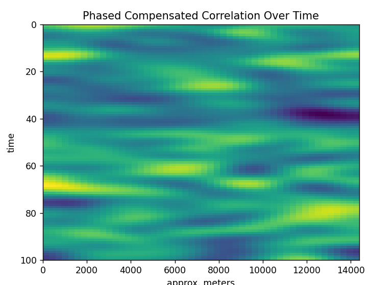
This is interesting. I’ve subtracted out the average per column. That leaves just the dynamic processes showing through. Who knows what that is. I’m using just a plain omni-directional antenna. I’ve used 2D gaussian smoothing to knock out the high frequency.
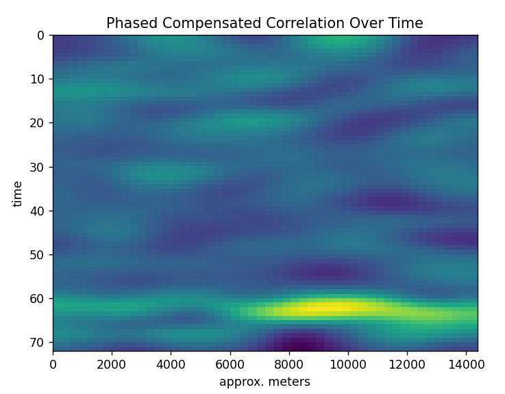
I like this one. It makes you wonder what that is that made the yellow spot. If the correlation was high the color is yellow, so something correlated really well at that specific time in which distance is a function of time. It even has a little twirl with it like it was changing altitude and present for a few measurements and then disappeared.
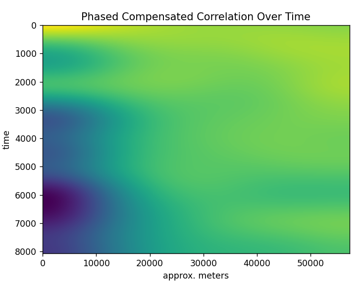
The (above) is a run over a few hours with some very heavily gaussian filtering on the vertical axis and lighter on the horizontal. This test was done with two log periodic antennas aimed at the sky – one transmit and one receive.
You can see some interesting changes over time. It appears that at first there is a lot of reflection near the ground and as time goes on the chirp penetrates further into the sky.
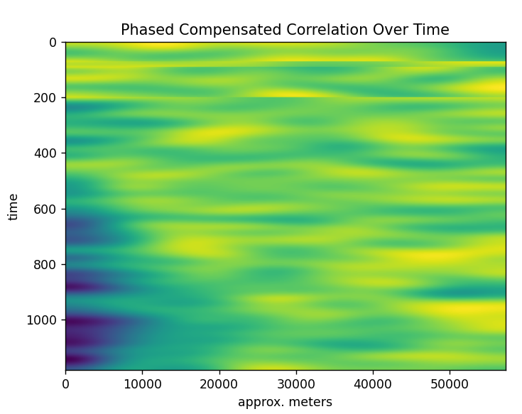
A higher resolution version but with more noise. I like this one because it seems to show some unique features for the column of sky being scanned. You can see the reflective base of the atmosphere rise over time. The falloff has been greatly compensated for with an average subtracted out down the Y axis so that only deviations from the average are shown. I wonder if some of those dips down low are clouds or cloudy skies passing by?
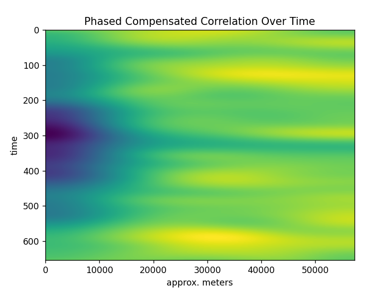
This is the same image, but the time period is about 12 hours now give or take. The ascending reflectivity base has now descended again. I will have to watch it over a longer period of time to see if this is a daily type of cycle.
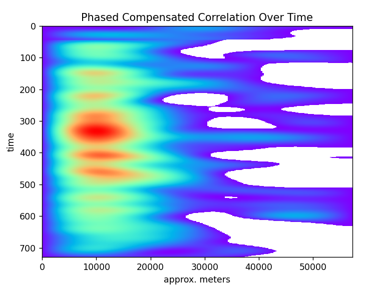
In this image (above), I’ve subtracted the along the X axis the previous measurement creating the amount of change from point to point. The white areas are negative which is where the reflectivity was decreasing with altitude/distance. This transformation of the data has revealed multiple regions of interest.
The first is from around 4e3 meters up to 20e3 where the reflectivity increases the fastest. Another set of areas are where the reflectivity is descending and then starts to ascend again as if the signal traveled through a region of significantly less reflectivity.