I was working on a long-term project to try to see if I can get a direction and distance from a two-element array. The following is what I’ve come up with and how I think it is working. It requires some testing, but it does follow some basic principles.
The Code
while True:
    samps = 1024 * 1024
    # How you get the samples can vary but in this case I'm
    # getting two channels of complex valued samples. You
    # might be using a BladeRF, a USRP, or something other.
    rxa_tx.put(samps)
    _, sa, sb = rxa_rx.get()

    for _ in range(1024):
        # Randomly choose some frequency within our baseband.
        lfreq = np.random.random() * sps - sps * 0.5

        # Filter as narrow of a band as possible.
        lsamps = abs(int(sps / lfreq))
        t = lsamps / sps
        w = np.exp(1j * np.linspace(
            0, np.pi * 2 * lfreq * t, lsamps
        ))
        fa = signal.convolve(sa, w, mode='valid')
        fb = signal.convolve(sb, w, mode='valid')

        # I just cut them to make grp_sz an integer multiple.
        fa = fa[:1000000]
        fb = fb[:1000000]

        # The phase difference.
        theta = np.angle(fa * np.conjugate(fb))

        # The size of each group. This is how many samples
        # we average.
        grp_sz = 100000
        assert len(theta) % grp_sz == 0
        # This is how many segments/groups we have to average.
        grps = int(len(theta) // grp_sz)

        # Each stream with magnitude taken, grouped into
        # segments, and these segments averaged.
        fa = np.mean(
            np.abs(fa).reshape((grps, grp_sz)), axis=1
        )
        fb = np.mean(
            np.abs(fb).reshape((grps, grp_sz)), axis=1
        )
        # The phase difference between antennas, grouped
        # into segments, and these segments averaged.
        theta = np.mean(theta.reshape((grps, grp_sz)), axis=1)

        # Get the actual frequency.
        afreq = lfreq + freq
        # Compute the antenna distance in meters. I'm using
        # the antenna distance on the BladeRF A4. This may
        # be different.
        ant_dist = 10 / 16 * 0.0254
        # Get the wavelength of the actual frequency.
        wl = 299792458.0 / afreq
        # The antenna distance in radians.
        ant_theta_dist = ant_dist / wl * np.pi * 2
        # The distance the wave saw between the antennas if
        # it was coming from an angle, broadside, or from
        # one of the ends.
        step_dist = theta / ant_theta_dist * ant_dist
        # The geometric angle the wave arrived at.
        geo_theta = np.arcsin(theta / ant_theta_dist)
        # I originally and wrongly did the below. This
        # according to my tests is not correct and it
        # makes sense why.
        # geo_theta = theta / ant_theta_dist * np.pi * 0.5

        # The two equations governing what the magnitude
        # should be from a wave originating at distance
        # `d` with a power level of `p``.
        # fa[x] = 1 / d ** 2 * p
        # fb[x] = 1 / (d - step_dist) ** 2 * p

        # The two equations solved for.
        E = step_dist ** 2 * fb
        d0 = (1 + np.sqrt(1 - 4 * E * fa)) / (2 * fa)
        d1 = (1 - np.sqrt(1 - 4 * E * fa)) / (2 * fa)

        # The first vector using the geometric angle.
        vec0 = np.exp(1j * geo_theta)
        vec1 = vec0.copy()
        # The second vector, mirrored, because of the
        # linear array.
        vec1.real = -vec1.real

        # The four solutions produced from each of the vectors
        # and each of the distance solutions.
        a = vec0 * d0
        b = vec0 * d1
        c = vec1 * d0
        d = vec1 * d1

        # The results dumped to a file.
        pickle.dump((a, b, c, d), fd)
Explanation
So, the idea is to grab some samples. Then create a very tight convolutional filter which should bring out a single frequency. Next, calculate the phase delta (two antennas) per sample. Take that phase delta and average it over some number of samples and do the same for the signal magnitudes at each antenna.
Since it is a two-element array there is ambiguity on the direction. In reality, there is a lot of ambiguity, but we can say the signal came from two pre-dominant directions but only one is the true direction. I’m going to handle that case towards the end.
In actuality there is some verticality in the direction, but you can’t detect that using just two elements. That leaves just the two pre-dominant directions I’m talking about. It also means that there would be additional error introduced for signals arriving with verticality onto the array which is going to manifest in the calculations below.
The step_dist is the distance that antenna B is from antenna A based on the angle of incidence; which is derived from the phase delta and linear antenna distance. It can be negative or positive depending on which side the wave was coming from. The geo_theta is the geometric angle of incidence, which is literally zero for broadside, -PI for arriving at antenna B first, or +PI for arriving at antenna A first.
Next, we solve the inverse distance problem. We know the two magnitudes of the signal at each antenna. We know the distance each antenna was from the other regarding the wave incidence angle, but we don’t know the power of the source nor the actual distance. This produces two equations (shown below) for each antenna and using some algebra and substitution we can reduce that to a single equation.
# The variable d and p are unknown.
fa[x] = 1 / d ** 2 * p
fb[x] = 1 / (d - step_dist) ** 2 * p

# Using algebra solve one equation for p and substitute
# into the second equation. Then use algebra to put into
# a quadratic form and solve below.
# ....

# reduces to the quadratic equation
E = step_dist ** 2 * fb
d0 = (1 + np.sqrt(1 - 4 * E * fa)) / (2 * fa)
d1 = (1 - np.sqrt(1 - 4 * E * fa)) / (2 * fa)
Taking this single equation which has power eliminated we have solved for distance. This single equation turns out to be a quadratic equation which can be solved using the quadratic equation – but we get two possible answers.
Now, we have two possible distances and two possible geometric angles which leads to four possible solutions: a, b, c, and d. Of course, most of the work was done in Numpy so these are arrays.
The arrays are of complex numbers, and these are the specific coordinates in meters where the real axis could be X and the imaginary axis could be Y or vice-versa. These are Cartesian coordinates.
Outputs
It gives some interesting outputs.


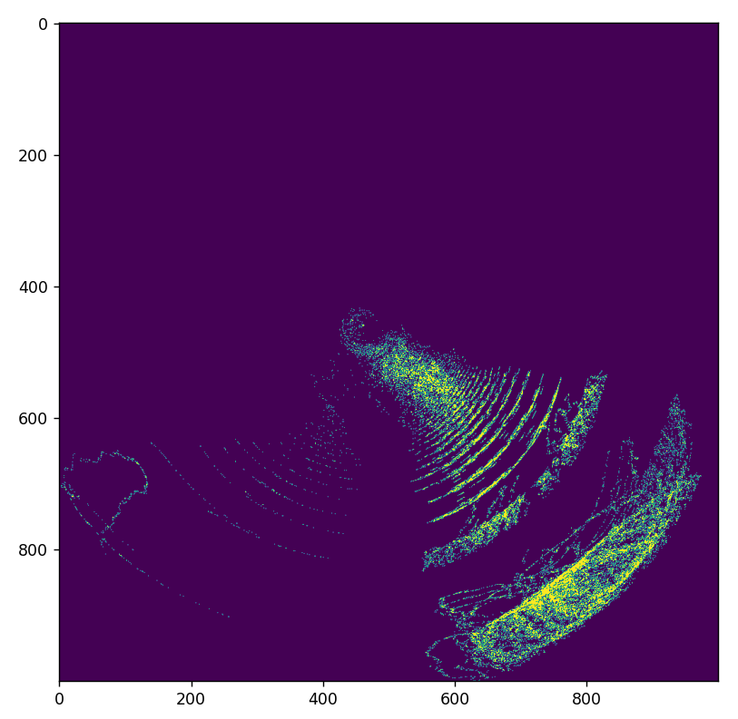
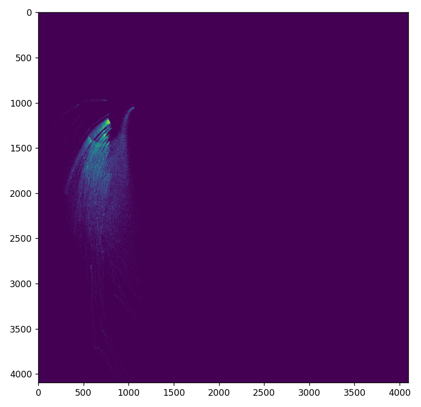
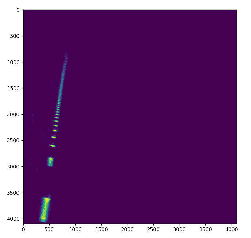
The above image looks like it grabbed onto something at 1.83ghz. It has me wondering about the ripples. I suspect those to be reflections perhaps from the ground or the sky? It raises some interesting questions. Like, why are there no reflections from other objects off to the sides? Perhaps the magnitude of the signal decreases too much or the angle of deflection isn’t perfect enough.
Like I said earlier on, the correctness is questionable. It needs some real testing to determine if it does come up with the right answers.
Plot Viewer
Here is the program that I use to produce the images.
import matplotlib.pyplot as plt
import pickle
import numpy as np
import matplotlib

def iter_file_pickles(path: str):
    with open(path, 'rb') as fd:
        while True:
            try:
                yield pickle.load(fd)
            except EOFError:
                break

ii = iter_file_pickles('plot2')

vz = []
try:
    while True:
        a = ii.__next__()
        for x in [0, 2]:
            for _v in a[x]:
                vz.append(_v)
except StopIteration:
    pass

v = np.array(vz)

plt.scatter(v.real, v.imag)
plt.show()

x_min = np.nanmin(v.real)
x_max = np.nanmax(v.real)
y_min = np.nanmin(v.imag)
y_max = np.nanmax(v.imag)

x_min = min(y_min, x_min)
x_max = max(y_max, x_max)
y_min = x_min
y_max = x_max

x = (v.real - x_min) / (x_max - x_min)
y = (v.imag - y_min) / (y_max - y_min)

img_w = 4096
img_h = 4096
img = np.zeros((img_h, img_w), np.float32)

x = np.round(x * (img_w - 1)).astype(np.int32)
y = np.round(y * (img_h - 1)).astype(np.int32)

for i in range(len(x)):
    try:
        img[y[i], x[i]] = 1
    except IndexError:
        pass

plt.imshow(img)
plt.show()
Source Magnitude
I was tinkering about and realized it might be better to plot source magnitude. You can derive this from the distance you computed earlier. This is the magnitude the source would have needed to be to produce the magnitudes on the two antennas using the square inverse law.
source_magnitude = fa / (1 / d0 ** 2)You have to pick from d0 or d1 which were the two solutions to the quadratic equation. I choose d0 because it usually seems to be the right answer.
This just looks better on plots.