This is a continuation of the previous tests and experiments.
Experiment A
Parameters: sps=520834, factor=1, samps_factor=1, sig_mag=200, tx_gain=42, rx_gain=60, bw=400e3The base sampling rate is sps but it is multiplied by factor. The base signal length in samples is 400,000 and it is multiplied by factor then divided by samps_factor. The two chirps are (-bw * 0.9, 10e3) and (10e3, bw * 0.9) which splits them across the spectrum each ascending in frequency thus maintaining a constant distance in frequency.
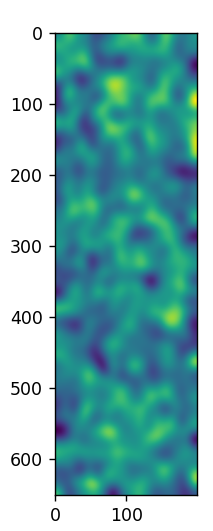
The above image is the correlated phase of the first signal with a Gaussian filter of sigma 10 applied.
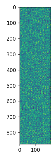
The above image is the raw phase output. The image received some smoothing from being displayed both during the screenshot and likely from being included in this page. Each horizontal row is a scan/correlation over time.
The data is very noisy looking but there are features that do not appear to be noise. These features stand out in the Gaussian filtered data.
Experiment B
Parameters: factor=2Here the factor was changed to 2 increasing the sampling rate and increasing the signal sample count. This kept the signal at the same duration and hopefully total power.
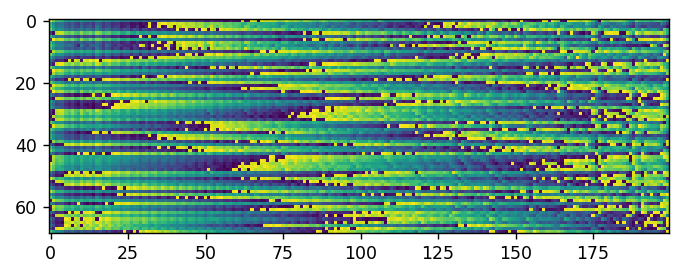
In this output, there is a repetition forming. The repetition is roughly 80 samples. Here there is much less noise and features are forming but they still have noise or at least each repetition has more noise. There appears to only be about two repetitions but there are more they were just truncated out of the data by the acquisition program.
Experiment C
Parameters: factor=4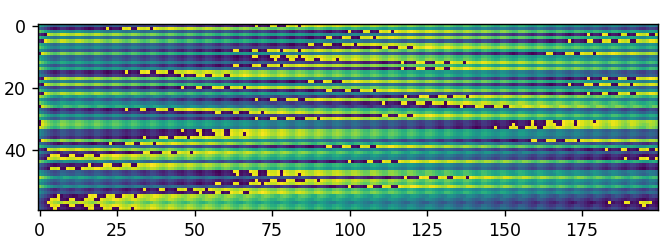
The repetition is not very visible if at all. During the past few experiments storms clouds have been increasing and the rain has started. The repetition may be hidden because it is longer than the 200 samples being displayed.
Experiment D
In this experiment the number of correlation samples displayed will be increased from 200 to 1000 and denoted by the parameter out_count.
Parameters: factor=8, out_count=1000
The repetition is clear to see. The width of each repetition is about ~406 samples. If the data is Gaussian filtered then truncated to 406 samples the output is below.

It should be noted the data being displayed is in phase with dark blue a negative phase and yellow a positive phase. If one was to imagine what the data could depict it might be the structure of the atmosphere passing overhead.
At a sampling rate of 4,166,672 (with factor of 8; 8 multiplied by 520,834) and a sample count of 406, speed of light at 299e6, then the total distance traveled at that speed would be 29,134 meters and halving the distance for a reflection (half-trip) would be 14,567 and dividing that by 1.6e3 (meters per mile) yields 9.1 miles.
It is impressive to think that ~10mW of power would reach 9.1 miles into the sky. It may be too impressive. This is exciting but requires further study to determine.
It is important to think about what happens to the phase as the signal travels and reflects. If the impedance of the medium increases the phase will be reversed and if the impedance is lower the phase (electrical) will not reverse. With this in mind as the signal travels it will continuously reflect energy as it encounters the medium along the way and it would seem correct to assume that this is what is being viewed. That lighter blue areas signify places where the signal did not invert because it was passing through similar or lesser reflective mediums such as plain air and in places where the output is yellow the signal was entering into more dense air mass with a higher reflectivity perhaps one with more water vapor. It is important to consider that the signal does not simply stop when it reflects. A portion of the signal continues moving and a portion reflects therefore further reflections would be from the unaltered original signal as it continues moving through the atmosphere.
One issue is that this may only be a display of impedance change and not actual reflectivity or total reflectivity. One way to gain that insight may be to use a formula of the sorts: np.sign(phase) * magnitude. This is because the phase appears in the data to start off negative (clockwise) and then it appears to move counter clockwise and become positive as the medium increases in impedance. This might give a interesting visual composition of the beam as it travels upward. The below image is the output.
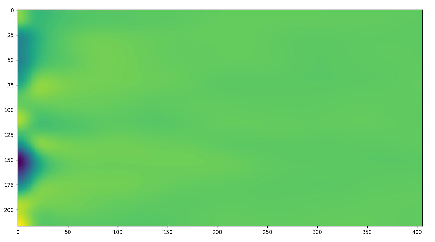
I am not certain of the accuracy. I think the decay of the signal is not being removed from the magnitude which is going to cause an inaccuracy in the visualization.
An improved idea is to consider the data of the shape (scan_index, sample_index) and then to take the mean of each sample column. A sample column is the array of samples at a particular sample_index across all scan indices. This would yield the decay curve and then to re-amplify the data of further samples out by dividing this decay curve into the magnitude. The output of that is shown below.
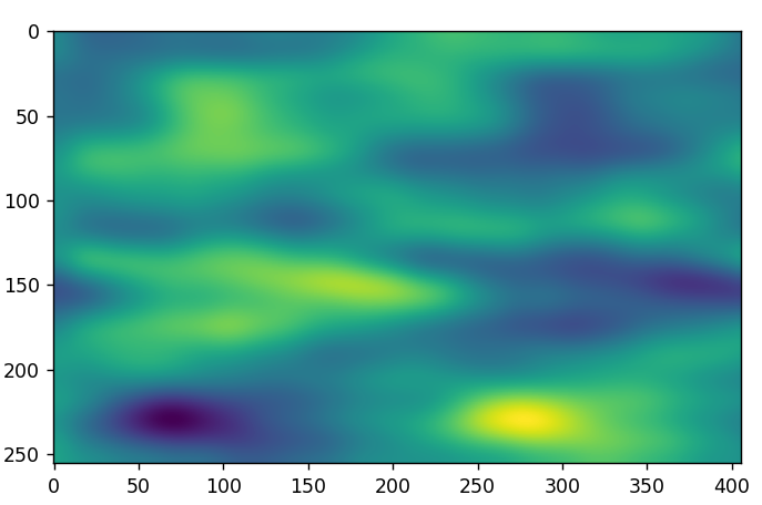
The output is very interesting.
Experiment E
For the previous experiment output I have been using a single linear chirp from a single transmit antenna. Yet there were two transmitted each one a separate antenna. There must be some interesting information encoded by the reflections with these two signals.
I should start with a thought experiment. I believe from some poking around the correlation is not yielding the same phase for each signal and perhaps this makes good sense since each signal originated from a different location therefore it wouldn’t be logical to assume they would be the same.
I also must confess that I’m confused about the phase of the reflections. It would seem to me that the distance the signal traveled would influence its phase since the phase of the signal upon arrival would be dependent on the distance. This means in my experiments taking the raw phase without some correction seems wrong. While it would make sense that it would represent reflectivity it would also make sense that the phase would be incorrect.
First, I should define a velocity of phase change. This should be equal to the velocity of the wave itself such that the phase makes a complete cycle for every wavelength. To calculate the expected phase I should be able to take the time of flight and divide this by the wavelength and then multiply it by PI*2.
Both images have Gaussian smoothing applied. The image on the left is the raw phase and the image on the right has the correction applied. I used a wave frequency of 400e3-hertz. I was not sure if I needed to use the baseband frequency, or the baseband frequency offset so I used the baseband frequency offset. It made some minor adjustments because some areas are better defined, and some regions have disappeared and changed.
The correction was calculated as phase_traveled = np.exp(1j * (299e6 / sps * np.linspace(0, c0.shape[0], c0.shape[0]) / wl * np.pi * 2)) where wl is the wavelength as 299e6 / 400e3. This was multiplied by the raw phase to correct or rotate it clockwise by the factor. The distance traveled is 299e6 / sps * c0.shape[0] which is a per sample distance. The rest converts it to the expected phase if it was reflected without any phase inversion. The c0 is the Numpy array of complex128 values representing the correlation output for the first linear chirp.
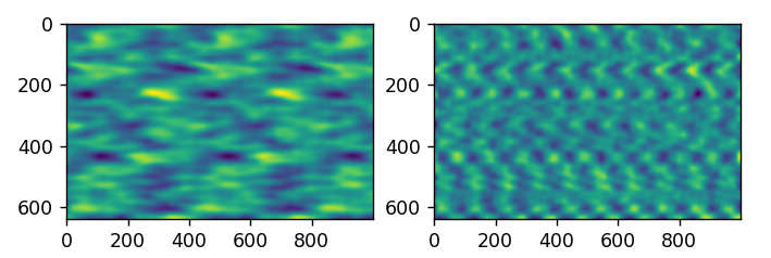
Of course, it does not appear to work. It rippled up the output and this seems to say to me that my idea of what I expected the phase to be was incorrect. However, let me try by the baseband frequency and see if there is any difference.

The above is using the baseband frequency of 3,449,262,038-hertz. It still produces ripples but it did break up the repetition. I tried the conjugate which produced the below.
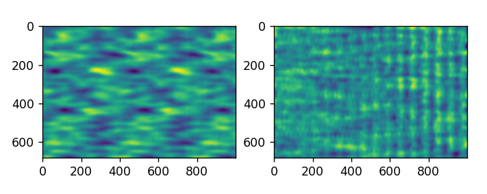
This gave ripples along the right side. I also must admit the repetition is still unexplained except for the hypothesis that it is bouncing the ground and going back up again.
The problem here is that without intimate understanding of how exactly phase works it is difficult to integrate the two signals correctly.
Now, I did notice that both my signals appear to be somewhat of an inverse of each other.
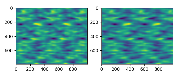
The first chirp (-bw * 0.5, 10e3) is on the left and the second chirp (10e3, bw * 0.5) is on the right. If one looks closely the features are reverse from right to left.
Summary F
At this point, I’m working with understanding why I get what phase readings I get from the correlation regarding the real-world signal traveling through a physical channel. In other words, while understanding the numerical correlation operation is a simple matter I’m dealing with complications involving two mixers, TX stage, RX stage, and an actual signal leaving an antenna, being affected by the physical channel, and then arriving in a separate, different type, antenna. While the process may be very simple, I’m not getting what I expect.
For example, one major expectation was that the signal would potentially undergo a phase shift simply from traveling in free space yet I’m not able to verify that behavior as correct. The second complexity is understanding exactly what is and is not happening within the mixer circuitry and antenna itself which likely contributes to what phase I transmit and what phase I see. Then, of course, the physical channel itself, if working correctly, should impact phase inversions and potentially, yet once again not proven to myself, phase shifts from reflections/impedance-changes.