I was thinking today about the propagation of an electromagnetic wave and specifically the phase velocity. I was pondering about how the phase velocity is dependent on frequency, and I decided to do a little test. I had done some previous experiments with sending out a chirp and listening for it to come back and I was wondering if phase velocity might have been a factor.
So, I wrote the best simulation I could of a discrete signal being transmitted and then received along with the phase velocity being a factor. I was able to determine that it had not been a factor because the distance wasn’t large enough.
I also think it is interesting how the velocity of a wave is different through the vacuum of space. You can find this happening with pulsars. You can read about that at Dispersion (optics) – Wikipedia.
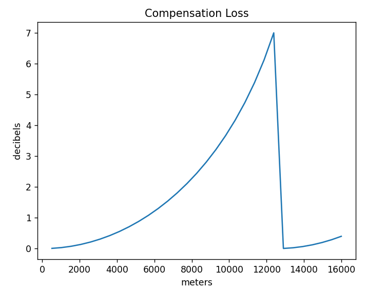
Here is the little program to simulate the gain in decibel when compensating for the phase shift per frequency over distance.
import numpy as np
import scipy.signal as signal
import matplotlib.pyplot as plt
import scipy.fft as fft

class AntSim:
    def __init__(self, sps, samps):
        self.wave_velocity = 299792458.0
        self.sps = sps
        self.samps = samps
        self.ant_locs = []
        self.ant_sig = []

    def add_ant(self, x, y, z):
        self.ant_locs.append(np.array([x, y, z]))
        self.ant_sig.append(np.zeros(self.samps, np.complex128))

    def do_signal(self, x, y, z, center_freq, signal):
        signal_pos = np.array([x, y, z]).astype(np.float64)

        sample_dist = self.wave_velocity / self.sps

        for ndx, ant_loc in enumerate(self.ant_locs):
            pos_vec = signal_pos - ant_loc
            dist = np.sqrt(np.sum(pos_vec ** 2))
            #print('dist', dist, pos_vec)
            sample_delay = dist / sample_dist
            sample_whole_delay = int(sample_delay)
            sample_frac_delay = sample_delay - sample_whole_delay

            #print('sample_delay', sample_delay)

            # How much room is left in the buffer. The rest of the
            # signal just flies on past.
            left = len(self.ant_sig[ndx]) - sample_whole_delay

            # This is weird looking but I really feel like it
            # follows the laws of physics. Each sinsusodial is
            # going to arrive at a different phase.
            new_signal = phase_shift_signal_by_distance(
                self.sps, center_freq, signal, dist, self.wave_velocity
            )

            #new_signal = signal

            # The attenuation if radiated from an isotropic source.
            attn = 1 / dist ** 2

            if left > len(new_signal):
                left = len(new_signal)

            self.ant_sig[ndx][sample_whole_delay:sample_whole_delay+left] += new_signal[0:left] * attn

def phase_shift_signal_by_distance(sps, center_freq, signal, dist, wave_velocity):
    fdom = fft.fft(signal)
    fdom_freqs = fft.fftfreq(len(signal), 1 / sps)
    phase_distance = dist / (wave_velocity / (fdom_freqs + center_freq)) * np.pi * 2
    # NOTE: I'm not certain if phase_distance is correct
    # or it should be negative.
    fdom *= np.exp(1j * phase_distance)
    return fft.ifft(fdom)

def main():
    sps = 24000
    center_freq = 1.83e9
    dist = 0 #50000000
    fbeg = -5000
    fend = 5000

    dist_space = np.linspace(0, 1600 * 10, 32)

    last_db = None

    # If you think this is weird wait until you find out
    # that different frequencies travel at different
    # velocities through a vacuum.
    # https://en.wikipedia.org/wiki/Dispersion_%28optics%29#Pulsar_emissions

    r = []

    for dist_off in dist_space:
        ant_sim = AntSim(sps, sps * 10)
        thetas = np.linspace(fbeg, fend, 20000) / (sps * 0.5) * np.pi * 2
        thetas = np.add.accumulate(thetas)
        chirp = np.exp(1j * thetas)

        ant_sim.add_ant(dist + dist_off, 0, 0)
        ant_sim.do_signal(0, 0, 0, center_freq, chirp)

        a = np.max(np.abs(signal.correlate(ant_sim.ant_sig[0], chirp, mode='valid')))

        chirp_shifted = phase_shift_signal_by_distance(
            sps, center_freq, chirp, dist + dist_off, ant_sim.wave_velocity
        )

        b = np.max(np.abs(signal.correlate(ant_sim.ant_sig[0], chirp_shifted, mode='valid')))

        db = np.log10(b / a) * 10
        r.append(db)

    plt.title('Compensation Loss')
    plt.ylabel('decibels')
    plt.xlabel('meters')
    plt.plot(dist_space, r)
    plt.show()

if __name__ == '__main__':
    main()
The results are significant because it shows, if I am correct, that at around 5290 meters I’ve losing a decibel of correlation response. I had my suspicions this might be a problem. I will need to perform some actual experiments to known for certain if I am correct.
In essence, what happens is the individual pure frequencies that make up the complex wave form arrive out of phase from when they were transmitted, and the correlation has to make up for that fact.

I should note that I’m not completely certain I’ve got the simulation correct. I’ve noted in the source where I’m iffy about if the phase should have been positive or negative and I’m also a bit worried if successive samples after sample zero are handled correctly. I plan to update this page if I find out it is incorrect.