In my previous page, BladeRF: Two Board Synchronization with Two Element Beamforming, I talked about and showed how to determine the beam angle for a two-element linear array. I showed how to get the beam angle to a single transmitting element and to a multi-element array. Finally, I showed an interesting way to probe out the best TX theta.
Here I want to show how to produce a beam that focuses on each antenna of the TX array and then how to send and recover two spatial data streams. This will be two data streams using the same frequency and time slot. If you are new to beamforming, then you might think it to be impossible because how does one transmit two different recoverable data streams using the exact same frequency at the exact same time?
To make this work we need to incorporate a weight for each antenna/element along with the theta. However, first we should have some intuitive understanding of how the weights change the beam.
I mentioned incorporating a weight. We already had a complex value but its magnitude was one. By weight I meant varying the magnitude. Later on, I learned what this really did is called spatial tapering. Check out the page below for a better description.
Beamforming & DOA | PySDR: A Guide to SDR and DSP using Python
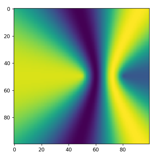
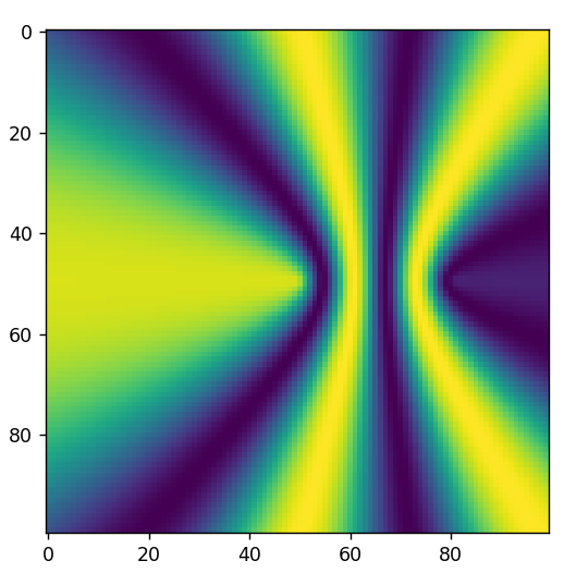
To do this we can simulate the reception of a signal from different points in space and then draw this image for visualization purposes. I’ve created two antenna/elements and positioned them 10/16-th of an inch apart on the X-axis and then I’ve taken a signal and moved it about in square. Then, I’ve plotted the results.

Frequency is fundamental because if the frequency is too high compared to the spacing between elements you can get more than a PI of phase difference and that creates fingers that spread outward making the pattern not have very good directional. The way to calculate wavelength is with speed_of_light / frequency and this should equal or exceed the antenna spacing distance.

In the above graphic, you can see the appearance of extra lobes. This happens because now the wavelength is less than the antenna spacing, and the directionality of the array suffers.
Another important fact is that the weight per element not only has an angular component but can have a magnitude. The interesting effect is that this controls the amplitude of each signal in the summation. Now, if you modify the amplitude of the two weights and plot the results you will notice it has near zero effect on the beam pattern. It does affect the total magnitude but the pattern itself is unaffected.
I believe in essence what is happening is that we are considering the case that each antenna receives the exact same signal and also considering that each antenna receives noise proportionally from each noise source. Yet, in a realistic setup not only does thermal noise affect each antenna differently but field patterns from noise may not affect each antenna equally.
In other words, one antenna may receive less noise, more of the signal, or both than the other. There may be a better SNR depending on which antenna you choose. I believe this is known as a rudimentary form of beamforming. In essence, you could just choose from one of the two antennas to receive the signal and pick the one with the best SNR.
However; it may be the case that a complex set of weights can choose a mixture of the two antennas with an associated phase shift on one to coax out the signal of interest in a constructive and deconstructive manner.
Another way to think about it is that with a simplistic view of a single noise source. Say some interfering signal. A simplistic view would say that the field moving away from this point source would have a uniform falloff and so it would appear as a spherical emanation but in reality, there are reflectors and attenuators all around in the real world causing the field pattern of this noise point source to be distorted in such a way that there are areas with more or less interference.
Not only that but there may be multiple sources of noise at the same frequency and these all interact in a complex way across space and time to create patterns that may not envelope both antennas equally.
So, sometimes not only does one antenna have better SNR but a mixture of each antenna can produce a better SNR. By mixture I mean the weight amplitude for both antennas can vary such that the range for a vector of weights might be:
[np.exp(1j) * np.random.random(), np.exp(random_theta) * np.random.random()]
If you notice in the above weight vector the magnitude of each antenna contribution to the final signal can vary along with the phase shift. I also modified the magnitude of the first weight and did not hold it at a magnitude of one.
The reason I think this way about it is because I’ve done some tests. I’ve tried simply switching one of the antennas off and using a single antenna, keeping the weight magnitudes at one, and varying the magnitudes of each weight. The best SNR was achieved when varying the weights like shown above.
I would call it a cross between a rudimentary version of beamforming where you select from the best antenna and actual phase shifting beamforming.

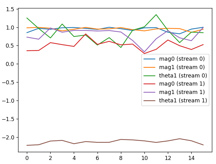
In the above graphic, I’ve plotted the results of a test. I’ve sent a number of transmissions back-to-back. Then, I’ve decoded each transmission and searched for the best possible SNR by varying the weights. Each transmission is two spatial digital amplitude modulated signals. I’ve labeled each spatial signal as steam 0 and stream 1 and the corresponding weight parameters. You do not see a theta0 parameter because the first weight’s angle is kept at zero since varying two thetas is equivalent to varying a single theta with two elements – maybe with more elements but not sure.
What is interesting is that a better SNR is found when the magnitude is allowed to vary for both elements. You can see that stream 0 performed well with both magnitudes near maximum but at times bringing in more of the second antenna into the summation/mixture produced a better SNR. Then for stream 1 the second antenna was a dominating factor.
To search for each of the signals, I used 6-bits of training symbols or a preamble and I made this preamble different for each stream. Then, I randomly probed out a set of weights that caused a correct decoding of the preamble. I ignored the four bits of data after the preamble but I did include a cause in the program to print out the exceptional condition that a correct preamble was found but the data was incorrect.
import argparse
import socket
import threading
import queue
import yaml
import pickle
import bladerf
import random
from lib.bladeandnumpy import BladeRFAndNumpy

def tx_thread(dev, num_buffers, buffer_size, freq, lo_freq, theta, sps, q, qout, sym_time, data_a, data_b):
    dev.sync_config(
        bladerf.ChannelLayout.TX_X2,
        bladerf.Format.SC16_Q11,
        num_buffers=num_buffers,
        buffer_size=buffer_size,
        num_transfers=8,
        stream_timeout=20000
    )

    for ch in [1, 3]:
        dev.set_gain_mode(ch, bladerf.GainMode.Manual)
        dev.set_bias_tee(ch, False)
        dev.set_frequency(ch, freq)
        dev.set_bandwidth(ch, sps)
        dev.set_sample_rate(ch, sps)
        dev.set_gain(ch, 35)
        print('tx-gain', dev.get_gain(ch))
        dev.enable_module(ch, True)

    buffer_samps = int((num_buffers * buffer_size) // 8)

    assert sps % lo_freq == 0

    samps = int(sps / lo_freq)
    samps = samps * int(buffer_samps // samps)
    t = samps / sps

    def build_tx_data(theta0, theta1):
        base = np.exp(1j * np.linspace(0, np.pi * 2 * lo_freq * t, samps))
        tx_data2 = np.zeros((len(base) * 4), np.int16)

        if theta0 is not None:
            tx_data0 = base * np.exp(1j * theta0)
            tx_data0 /= np.max(np.abs(tx_data0))
            tx_data0 *= 2000
            tx_data2[0::4] = tx_data0.real
            tx_data2[1::4] = tx_data0.imag
        else:
            tx_data2[0::4] = 0
            tx_data2[1::4] = 0

        if theta1 is not None:
            tx_data1 = base * np.exp(1j * theta1)
            tx_data1 /= np.max(np.abs(tx_data1))
            tx_data1 *= 2000
            tx_data2[2::4] = tx_data1.real
            tx_data2[3::4] = tx_data1.imag
        else:
            tx_data2[2::4] = 0
            tx_data2[3::4] = 0

        tx_data = tx_data2.tobytes()
        return tx_data

    print('tx thread going')

    # Start with both antennas OFF by sending all zeros.
    tx_data = build_tx_data(None, None)

    while True:
        try:
            msg = q.get_nowait()
            if msg is True:
                break
            theta0, theta1 = msg
            print('tx change', theta0, theta1)
            tx_data = build_tx_data(theta0, theta1)
            qout.put(None)
        except queue.Empty:
            pass
        dev.sync_tx(tx_data, int(len(tx_data) // 4))

    def build_bits(bits_a, bits_b):
        bit_stream = np.repeat(bits_a, sym_time)
        t = len(bit_stream) / sps
        base = np.exp(1j * np.linspace(
            0, np.pi * 2 * lo_freq * t, len(bit_stream)
        ))

        a = base * bit_stream * 2000

        bit_stream = np.repeat(bits_b, sym_time)
        b = base * bit_stream * 2000

        #with open('plot', 'wb') as fd:
        #    pickle.dump((a, b), fd)

        tx_data = np.zeros(len(a) * 4, np.int16)
        tx_data[0::4] = a.real
        tx_data[1::4] = a.imag
        tx_data[2::4] = b.real
        tx_data[3::4] = b.imag

        tx_data = tx_data.tobytes()

        return tx_data

    print('building bits')

    tx_data = []

    seq = [0, 0]
    for x in range(8 * 10):
        tx_data_seg = build_bits(data_a, data_b)

        for y in range(3):
            tx_data.append(tx_data_seg)

    tx_data = b''.join(tx_data)

    qout.put(None)

    while True:
        try:
            msg = q.get_nowait()
            bits_a, bits_b = msg
            tx_data = build_bits(bits_a, bits_b)
            qout.put(None)
        except queue.Empty:
            pass

        dev.sync_tx(tx_data, int(len(tx_data) // 4))

class TrainingSymPrefixDecodeAM:
    def __init__(self, rx_stream_count, sym_count, sym_samps, lo_freq, sps):
        self.sym_samps = sym_samps
        self.sym_count = sym_count
        self.samps = self.sym_samps * self.sym_count
        self.rx_stream_count = rx_stream_count
        self.sps = sps
        self.frame_samps = self.sym_samps * self.sym_count
        self.frame_time = self.frame_samps / self.sps
        self.lo_freq = lo_freq
        t = (self.sym_samps * self.sym_count) / self.sps
        self.signal = np.exp(1j * np.linspace(
            0, np.pi * 2 * self.lo_freq * t, self.samps
        ))
        self.best_w = [None] * self.rx_stream_count

    def decode_search(self, rx_streams, prefixes, exp_data=None):
        assert len(rx_streams) == len(prefixes)
        assert len(rx_streams[0]) == self.samps

        data = [None] * len(prefixes)

        self.best_snr = [0] * self.rx_stream_count

        # Track what streams have at least one successful decode.
        s_decoded = [False] * self.rx_stream_count

        st = time.time()
        rst = time.time()

        # Wait 20 seconds after last decode with a better SNR if all streams have
        # at least one decode done.
        while time.time() - st < 20 or not np.all(s_decoded):
            # Stop if we exceed 300 seconds with no new better SNR found.
            if time.time() - st > 300:
                print('failed to solve')
                return

            # Iterate through each expected stream.
            for x in range(len(rx_streams)):
                prefix_size = len(prefixes[x])

                # (1) Create a random weight vector.
                w = [np.exp(1j) * np.random.random()]
                for _ in range(len(rx_streams) - 1):
                    rtheta = np.random.random() * np.pi * 2 - np.pi
                    w.append(np.exp(1j * rtheta) * np.random.random())

                # (2) Multiply the weight vector by the signal streams.
                # This is the classic beamformer equation. This is the
                # summation and phase shift part.
                c0 = rx_streams[0] * w[0]
                for i in range(len(w)):
                    c0 += rx_streams[i] * w[i]

                # Filter out just the AM transmission frequency.
                c0 = np.abs(c0 * np.conjugate(self.signal))
                # Decode the AM transmission using averaging.
                c0 = np.mean(c0.reshape((self.sym_count, self.sym_samps)), axis=1)
                # Compute the binary ones and zeros. Stored as True and False.
                decoded = c0 > np.mean(c0)

                # Rotate the sequences until we find the preamble, IF we find it because
                # we may not.
                good = False
                snr = 0
                for _ in range(self.sym_count):
                    if np.all(decoded[0:prefix_size] == prefixes[x]):
                        # Calculate a signal to noise ratio.
                        snr = np.min(c0[c0 > np.mean(c0)]) - np.max(c0[c0 < np.mean(c0)])
                        good = True
                        if snr > self.best_snr[x]:
                            if exp_data is not None:
                                if not np.all(decoded == np.array(prefixes[x] + exp_data[x])):
                                    print('BAD DECODE')
                            self.best_snr[x] = snr
                            self.best_w[x] = w
                            print('BEST', x, self.best_snr[x], w)
                            data[x] = decoded[prefix_size:]
                            st = time.time()
                        s_decoded[x] = True
                        break
                    decoded = np.roll(decoded, 1)

        print(f'solved in {time.time() - rst} seconds')

        self.best_w = np.array(self.best_w)

        return data

def main():
    devs = []

    print('opening cards')
    for serial in ['9da', 'e85']:
        devs.append(BladeRFAndNumpy(f'libusb:serial={serial}'))

    sps = 1000000

    num_buffers = 16
    buffer_size = 1024 * 32
    buffer_samps = num_buffers * buffer_size

    print('configuring rx')
    devs[0].sync_config(
        bladerf.ChannelLayout.RX_X2,
        bladerf.Format.SC16_Q11,
        num_buffers=num_buffers,
        buffer_size=buffer_size,
        num_transfers=8,
        stream_timeout=20000
    )

    freq = 1.83e9

    # Pick a random frequency with an appropriate wavelength
    # that is not too small but still gives us as narrow of
    # a main lobe as possible.
    freq = random.randint(int(2e9), int(3e9))

    #freq = 3e9
    lo_freq = 20e3

    buffer_samps = int((num_buffers * buffer_size) // 4)

    q = queue.Queue()
    qout = queue.Queue()

    # This is the symbole time in samples. The modulation is digial AM and
    # I use averaging so increase the SNR so a larger sym_time should
    # translate into an increased SNR.
    sym_time = int(sps // 200)

    # This sets up the preamble and data components. A lengthly preamble seems to
    # work well. It may take some experimentation here to figure out what lengths
    # work the best for what data lengths.
    preamble_a = [0, 1, 0, 1, 1, 0, 0, 1, 0, 0, 1, 1]
    preamble_b = [1, 1, 1, 0, 0, 1, 1, 0, 1, 1, 0, 0]
    data_a = [1, 0, 1, 0]
    data_b = [0, 1, 1, 0]

    tx_th = threading.Thread(
        target=tx_thread,
        args=(
            devs[1],
            num_buffers,
            buffer_size,
            freq,
            lo_freq,
            0.0,
            sps,
            q,
            qout,
            sym_time,
            preamble_a + data_a,
            preamble_b + data_b
        ),
        daemon=True
    )

    print('started tx thread')
    tx_th.start()

    time.sleep(2)

    print('setting rx params')
    for ch in [0, 2]:
        devs[0].set_gain_mode(ch, bladerf.GainMode.Manual)
        devs[0].set_bias_tee(ch, False)
        devs[0].set_frequency(ch, freq)
        devs[0].set_bandwidth(ch, sps)
        devs[0].set_sample_rate(ch, sps)
        devs[0].set_gain(ch, 60)
        devs[0].enable_module(ch, True)

    samps = int(sps / lo_freq)
    samps = samps * int(buffer_samps // samps)
    t = samps / sps

    def clear_rx_buffer():
        a, b = devs[0].sample_as_f64(buffer_samps, 2, 4, 0)

    # Put the TX thread into the second mode which will send
    # amplitude modulated digital data.
    q.put(True)
    qout.get()
    time.sleep(1)
    clear_rx_buffer()

    # This is calibrated to my cards. It needs to be adjusted for your
    # cards. See my previous pages for synchronizing two boards to acquire
    # this value. It is created by the slight differneces in master clock
    # frequencies on the boards. This value might work for you thought your
    # milage just may vary.
    tx0_freq_off = -3937.0

    sym_count = len(preamble_a) + len(data_a)

    # The total number of samples in a single transmission.
    samps = sym_time * sym_count

    print('reading signal')

    tspdam = TrainingSymPrefixDecodeAM(
        2,                  # total streams/elements/antennas
        sym_count,          # total number of bits
        sym_time,     # symbol/bit duration in samples
        tx0_freq_off,       # transmitter offset/error
        sps                 # samples per second
    )

    # The transmitter is just repeating the transmission back to back
    # so we can grab as many as we like here. The decoder routine does
    # a roll on the decoded bits because it assumes the transmissions
    # are cyclic - which they are.
    iterations = 10
    sa, sb = devs[0].sample_as_f64(samps * iterations, 2, 4, 0)

    fd = open('plot', 'wb')

    for i in range(iterations):
        # Grab just one portion which is equal to a transmission size.
        a = sa[samps * i:samps * i + samps]
        b = sb[samps * i:samps * i + samps]

        print('MPWR', np.mean(np.abs(a)), np.mean(np.abs(b)))

        data = tspdam.decode_search(
            # These are the signal vectors.
            [a, b],
            [ # These are the preambles/training sequences.
                preamble_a, # preamble channel a
                preamble_b, # preamble channel b
            ],
            [ # This is the expected data for diagnostic purposes.
                data_a,
                data_b,
            ]
        )

        print('data', data)

        # Log the results to disk.
        pickle.dump(tspdam.best_w, fd)

if __name__ == '__main__':
    main()
In the above program, I’ve created a class that does the decoding and searching for the signals. The work method of the TrainingSymPrefixDecodeAM class is called code_search. In this method, a loop is used to randomly probe using different weights for each stream. The weights used are dumped to a file called plot which is the file that I plotted the last graphic from.
This program proves that two data streams can be received from two separate antennas even though both data streams use the same spectra/frequency. You should be able to place the BladeRF boards at a reasonable distance but mine for the tests were within a meter of each other.
You can also normalize the first weight’s magnitude to one using the equation 1 / first_weight_magnitude * second_weight_magnitude and this computes the second weight’s magnitude if the first weight was one. So, it is possible to keep the first weight’s magnitude at one. I just allowed it to vary because it bounded my space between 0.0 and 1.0 when searching for the weights. This means only the second weight element of the weight vector was required to be searched out like in classical beamforming texts.
Another interesting fact is that the somewhat optimal weight vector changes over time. It does have some consistency as one can see in the chart. If you plot out all the valid weight vectors you will see that there is a region within weight space where the valid vectors group together. This means at some points the same weight vector can be reused across different transmissions but to achieve the highest SNR it must change with the changing conditions of the environment.
I’ve also noticed that training it over more symbols produces a lower error rate for the data payload. I assume that this is because it forces it to find a more optimal weight vector solution that is more stable over a longer period. If I were to imagine the solution space for the weight vector, then I would see this space getting smaller as the number of training symbols increased and ultimately there would be some weight solution that would maximize the transmission length up to a certain point where noise/interference would become too much.
If you have problems getting it to work, try setting the frequency instead of using the random range or re-run the program to pick a new frequency. It is possible the frequency doesn’t have enough SNR because of noise, your antenna, or the distance between the boards. Also, check that your tx0_freq_off is set correctly to the error between the two boards. Each board has a slightly different sampling frequency, and it translates to a frequency error.